
In 1958, Joseph Youngblood's article entitled "Style as Information" explored the notion of musical style as a set of mathematically verifiable preferences for certain musical structures over others.1 In the study, he concentrated on single melodic pitches and consecutive pairs of melodic pitches in certain works by three composers of tonal music—Schubert, Mendelssohn, and Schumann—and rated the frequency of these structures in that early nineteenth-century style using the mathematical methods of information theory. One year earlier, Leonard Meyer, too, suggested information theory as an appropriate method for defining a given style.2 Much less mathematical and more descriptive than Youngblood in his approach, Meyer explains that (at least some) music has "embodied meaning," which arises, he says, when "within the context of a particular musical style one tone or group of tones indicates—leads the practiced listener to expect—that another tone or group of tones will be forthcoming at some more or less specified point in the musical continuum."3 Although he provides no examples, Meyer suggests the usefulness of mathematical approaches such as Youngblood's when he says, "Once a musical style has become part of the habit responses of composers, performers, and practiced listeners it may be regarded as a complex system of probabilities."4
Prokofiev's music is often said to be tonal, although it does not usually follow the norms of common-practice tonality. This study examines the melodies from Prokofiev's Romeo and Juliet as representatives of at least his later style, submitting them to information-theory calculations in order to compare this style with the early nineteenth-century style studied by Youngblood, and further exploring the style as "a complex system of probabilities" by submitting several aspects of the melodies to a chi-square test.
A couple of difficulties with such a mathematical analysis of these melodies must be dealt with at the outset. First, the results of the statistical tests reported below cannot be taken as impeccably dependable due to the impossibility of devising a truly random sample of data, or, in fact, of even determining the exact contents of the entire population. The difficulty is that the ultimate concern is not with discovering patterns that occur more often in actuality, but rather with those that seem to occur more often. If a given melody is repeated ten times over the course of a work, each pattern within that melody is itself heard ten times. Does any such pattern indeed seem ten times as normal as one found in a melody heard only once? Should the pattern occur in other melodies as well, the repetition of the first melody would seem to confirm the notion that the pattern is in fact an integral part of the whole style. But what of the comparison of a pattern that is found only in the ten-times-repeated melody with another that is found in five different melodies, each melody heard only once? The recurrence of the second pattern in five different contexts is likely to make it seem more normal than the pattern heard in only one context, despite the fact that the latter is heard twice as often. There can be no true resolution of this problem since any two listeners may approach it in different ways. Using V-I cadences and Tristan und Isolde as examples, Leonard Meyer has pointed out that it is possible, to a listener familiar with the norms of a particular body of literature, for a given pattern to seem an integral part of the style of a certain work even if no instances of it are heard in the work at all.5
Second, even if the methodology is allowed some leeway, an argument could be raised against using statistics in such a study: such methods often seem able to avoid being cold and inhuman only by being inexact and thus meaningless. As to the first possibility (that the methods ignore some human element in the music), any form of note counting can only be a first step in meaningful analysis. Subjective sense is always available, and indeed necessary, for interpreting findings. The purpose of this study is to compare Prokofiev's melodic style with that of earlier tonal composers by means of an established method, and the study proffered by Youngblood and its concomitant statistical methods provide the baseline for the comparison. So the concern of this study is indeed note counting, but the study is meant to be only a first step on one path toward understanding this music.
As to the second possibility, since the resolution of our subjective sense of what seems more or less normal is not nearly so refined as that suggested by the multi-decimal-place figures statistical computations produce, inexact figures should be enough for laying a basic foundation. In short, if the study is not expected to produce data complete enough and accurate enough, say, to drive a Prokofiev-imitating computer program, it can still be quite revealing.
Out of a total of forty-four different melodies in Romeo and Juliet, thirty-seven, those that begin and end in the same key, were included in the reckoning for this study, each of them counted only once. In a few cases, only major-mode melodies were counted. The location of each of these melodies is given in figure 1.6
Figure 1. List of melodies used in study.
| 1. Beginning: 1-4 2. 1:5-12 3. 1:13-20 4. 2:6-13 5. 6:3-7:1 6. 9:5-11:1 7. 18:5-19:8 8. 30:1-8 9. 44:5-8 10. 48:1-4 11. 50:1-8 12. 55:1-6 13. 60:1-4 |
14. 64:1-9 15. 67:1-4 16. 71:1-8 17. 73:1-4 18. 84:1-85:8 19. 88:3-89:10 20. 97:1-5 21. 106:1-8 22. 107:1-17 23. 111:1-112:8 24. 122:3-123:1 25. 125:2-9 |
26. 151:5-152:1 27. 152:2-153:1 28. 161:1-7 29. 174:9-19 30. 178:1-16 31. 201:1-4 32. 207:1-8 33. 208:1-209:8 34. 212:6-8 35. 213:5-214:8 36. 289:1-8 37. 315:3-6 |
Individual pitches (classification of pitch determined by its intervallic relationship to the prevailing tonic, hence the necessity for melodies that begin and end in the same key), contiguous two-note patterns, patterns of two notes separated by a third note, and melodic intervals were counted. Distributions of the tendencies were then subjected to chi-square tests to study their deviation from randomness, from other distributions provided by the same study, and from the distributions provided by Youngblood. In addition, Youngblood's method of information-theory computation was applied to these same distributions for further comparison with the nineteenth-century style he examined.
Explanation of Chi-square Test
The chi-square test is used to judge whether the difference between two nonnormal distributions is significant or not. In other words, given a nonnormally distributed set of probabilities (specifically, the probability for each possible value of a given discrete variable) as a basis for expectation, the chi-square test will determine, within a certain level of confidence, whether a set of observed frequencies could have resulted from those given probabilities. If not, a "significant" difference exists, and a factor other than chance can be assumed to have influenced the observed results.
The first step in this test is to subtract the observed frequency of each possible outcome from its expected frequency (the probability of that outcome multiplied by the total number of instances). The square of each difference is then calculated and divided by the corresponding expected frequency. The results are then totaled. This final figure is compared with figures in a chi-square table, which can be found in any statistics text. The table gives the minimum result needed to assume significance of deviation with confidence of a certain degree: 99%, 98%, 95%, etc. 99% confidence, for instance, means that the difference could have arisen by chance only one time in 100; the observer can be 99% sure that other factors, not chance, caused the difference. The table also gives different figures for varying degrees of freedom (df). For our purpose, the degrees of freedom is a number equal to the number of possible outcomes minus one. The notion of degrees of freedom reflects the interdependence of the frequencies of the various outcomes when the total frequency is given. If there are only two possible outcomes in a certain system and the total frequency is given, any result for one outcome determines the frequency of the other; there is only one degree of freedom in the system. If three outcomes are possible, the frequencies of any two outcomes are independent of each other, but the third is determined by the other two; there are two degrees of freedom. With greater degrees of freedom, higher chi-square figures are needed in order to determine significant deviation. Because the test involves dividing the square of each difference by the expected frequency, the fact that significance of deviation rises as the total frequency rises is taken into account. (Anything can happen once; probabilities take effect over multiple occurrences.) In the same feature, however, lies one weakness of the test: any expected frequency less than about 2% of the total frequency may, since it is used as a denominator, possibly lead to an overly large result.
As an example, let us imagine that for a given location, two-thirds of the days are sunny, one-third cloudy. The probability that any given day will be sunny is thus .67, that it will be cloudy, .33. Over a 30-day period, 20 sunny days would be expected, 10 cloudy days. An observation of 19 sunny days and 11 cloudy days would not seem unusual, and the chi-square test confirms that it is not so. The difference between the expected frequency of sunny days and the observed frequency is 1. The square of this difference is 1, and this divided by the expected frequency is .05. The difference for cloudy days is also 1. The square, 1 again, is divided by the expected number of cloudy days, for a result of .1. The sum of the results is .15. With one degree of freedom, a result of at least 3.841 is needed for even 95% confidence; the chi-square test indicates that only chance was involved in the deviation. Suppose, however, that 10 sunny days and 20 cloudy days were observed. This would be quite an unusual weather pattern for the location, as the chi-square test would affirm. The difference squared is, in each case, 100. Dividing 100 by the expected number of sunny days yields 5; dividing by the expected number of cloudy days gives a result of 10. Totalling these results yields a final chi-square figure of 15. Only 6.635 is needed for 99% confidence that a significant difference exists.
Explanation of Information-Theory Calculation
The information-theory calculation is also a summation of figures. For each outcome, the proportion of the observed frequency to the total number of events is multiplied by the log2 of that same proportion. (The log2 of a number is that power to which 2 must be raised to yield that number. 8 is 2 to the third power. Therefore the log2 of 8 is 3. 0.25 is 2 to the power of negative 2. Therefore, the log2 of 0.25 is -2.) The absolute value of the sum of these products yields the number of bits of information expressed by the system and is known as the entropy of the system, represented by the letter H. (A bit is the smallest amount of information, a binary choice, an indication of the state of a situation where only two possibilities exist. One bit of information is needed to indicate one of two objects. Two bits are needed to indicate one of four objects; the first bit narrows the field in half, and the second can then identify one of the two remaining possibilities. Three bits are needed to identify one of eight objects, etc.) Where the observed frequencies are the same for each possible outcome, the entropy will be the log2 of the number of outcomes. With four possible outcomes, for instance, the result would be 2. Where the frequencies are not equal, the theory states that less information is expressed by each event. Another way Youngblood explains it is that if a composition displays more instances of one possibility (a given pitch or rhythmic value, for instance) than another, the composer was less free to choose the rarer of the two. A lower entropy figure indicates less freedom of choice, more restrictions due to peculiarities of style. The entropy figure of a nonequally distributed system may be divided by the figure for an equally distributed system with the same total number of events to yield the figure known as relative entropy (Hr).
To demonstrate the information-theory or entropy test, I will relay Youngblood's example: a composer is writing a piece for four drums in which he uses drum A 12.5% of the time, drum B 12.5%, drum C 25%, and drum D 50%. The log2 of .125 is -3; of .25, -2; and of .5, -1. (.125 * -3) + (.125 * -3) + (.25 * -2) + (.5 * -1) = (-.375 + -.375 + -.5 + -.5) = -1.75. The absolute value is taken just for the convenience of having positive numbers as results. Thus H = 1.75. Since H would equal 2 in a system with four equally probable possibilities, Hr = 1.75/2 = .875 = 87.5%.
This method has two main weaknesses. First, there is no absolute standard for making judgments based on the results of this test, as there is in the case of chi-square. However, relative judgments may be made by comparing results and deciding which of two systems, for instance, displays more freedom of choice, i.e., which deviates from randomness less. Second, since only relative frequency and not absolute frequency is taken into account, the difference in significance that accompanies greater frequencies is not factored in. Getting "heads" only twenty-five times in one-hundred coin tosses is viewed by this theory as no less a product of chance than getting "heads" once in four tosses. Still, the method may be useful in corroborating findings from other tests.
Distribution of Individual Pitches
Before any multi-note patterns can be examined, the relative frequencies of pitches must be established. The distribution of frequencies of each pitch class as occurring in melodies 1-37 is shown in table 1.
Table 1. Frequency distribution of pitch classes in the Prokofiev melodies. PC designations are relative to tonic.
| PC 0 1 2 3 4 5 6 7 8 9 10 11 |
Relative Freq. 256 30 135 56 188 103 58 263 44 144 52 132 Total: 1461 |
Freq. 17.52% 2.05% 9.24% 3.83% 12.87% 7.05% 8.97% 18.00% 3.01% 9.86% 3.56% 9.03% |
The "PC" designation in the first column refers to the number of half steps a given note lies above the tonic pitch of the melody in which it occurs. Thus, there are 256 instances of the tonic pitch in these melodies, 30 instances of the pitch one half-step above the tonic, etc. (These pitch-classes will be indicated in the text from this point on as an underlined integer, e.g. 3.) "Relative freq." refers to the proportion of a given PC's frequency to the total number of pitches, in this case 1461. A pitch chosen at random from the melodies of this ballet then has an 18% chance of being the dominant pitch (7), but is only about half as likely to be the leading tone (11). The distribution is clearly not random; the chi-square test yields a result of 584.86, where for 99% confidence with 11 degrees of freedom, a result of only 24.725 is required. Thus, these frequencies are significant aspects of the style. The dominant and tonic, in that order, are the most common scale degrees, followed by the third, the sixth, the second, the seventh, and the fourth degrees of the major scale. As might be expected, the chromatic pitches are less common. The entropy of this distribution is 3.300. Since the H for twelve classifications with equal probabilities is 3.585, the Hr for this distribution is .921. Meaningless now, this figure will prove somewhat useful when comparing other distributions to this overall distribution.
Youngblood's study dealt only with melodies in major keys. For this reason a division by mode of the melodies in Romeo and Juliet is desired. Distributions for each mode are given separately in table 2.
Table 2. Frequency distribution of pitch-classes by mode.
Major mode
RelativeMinor mode
Relative
PC
0
1
2
3
4
5
6
7
8
9
10
11Freq.
211
26
107
31
184
92
46
185
23
126
17
112
Total: 1160Freq.
18.19%
2.24%
9.22%
2.67%
15.86%
7.93%
3.97%
15.95%
1.98%
10.86%
1.47%
9.66%Freq.
45
4
28
25
4
11
12
78
21
18
35
20
Total: 301Freq.
14.95%
1.33%
9.30%
8.31%
1.33%
3.65%
3.99%
25.91%
6.98%
5.98%
11.63%
6.64%
Not surprisingly, since it is the relative frequency of 4 and 3 which more than any other factor determines whether a melody is in the major or minor mode, in each mode here the appropriate third scale degree is found approximately six times as often as its counterpart. Also not surprising is that the minor mode employs the leading tone less often than does the major mode and employs the sub-tonic much more often. Of note is the much higher frequency of dominant pitches in the minor mode and the much lower frequency of the subdominant. The use of 6 just under 4% of the time in each mode is striking. As might be expected, the entropy figures for these distributions, 3.220 for the major mode (Hr =.898) and 3.189 for the minor mode (Hr = .890), are lower than those for all the melodies together. This is true because the strictures associated with each mode are isolated in the dual breakdown. In other words, the extra freedom indicated by the higher H value of the combined distribution represents the freedom to choose one of two modes.
We may now begin to compare the Prokofiev figures with those obtained in Youngblood's study. The H values for the three composers studied by Youngblood are as follows: Schubert, 3.127 (Hr = .87); Mendelssohn, 3.03 (Hr = .846); and Schumann, 3.05 (Hr = .85). Obviously, Prokofiev is more free in his choice of pitches than is any one of the three nineteenth-century composers. Schubert comes the closest, probably because he is the most chromatic of the three. An examination of differences between Prokoviev's choice of pitches and Schubert's may disclose specific ways in which the style of Prokofiev's music differs from an earlier tonal style. In table 3, Schubert's frequency distribution, taken from Youngblood, is given alongside Prokofiev's.
Table 3. Comparison of PC-probability distributions for Schubert and Prokofiev.
Schubert
RelativeProkofiev (major)
Relative
PC
0
1
2
3
4
5
6
7
8
9
10
11Freq.
182
7
168
23
124
83
16
203
30
78
29
82
Total: 1025Freq.
17.76%
0.68%
16.39%
2.24%
12.10%
8.10%
1.56%
19.80%
2.93%
7.61%
2.83%
8.00%Freq.
211
26
107
31
184
92
46
185
23
126
17
112
Total: 1160Freq.
18.19%
2.24%
9.22%
2.67%
15.86%
7.93%
3.97%
15.95%
1.98%
10.86%
1.47%
9.66%
Although it is clear which pitches Prokofiev uses more often than Schubert and which pitches less, the question at hand is whether any of the differences is significant. Assuming the proportions displayed for Schubert are typical, i.e., that they can be expected, are the discrepancies between the two composers possibly a matter of chance, or do they indicate significant differences in style? The chi-square figure obtained by a comparison of the full distributions is 170.895. With only 24.725 or greater needed for 99% confidence, it is clear that significant differences exist. What, specifically, are they?
The first issue is the matter of chromaticism. Of the 1025 notes examined in the Schubert study, 920 (89.8%) are diatonic, 105 (10.2%) chromatic. Of the 1160 notes in the major-mode Prokofiev melodies, 1017 (87.7%) are diatonic, while 143 (12.3%) are chromatic. The Prokofiev melodies thus display more chromaticism. Is the difference significant? The chi-square test suggests that it is. Given the Schubert percentages as the normal probabilities, the Prokofiev figures yield a chi-square value of 5.733. Since at 1 degree of freedom 5.412 is needed for 98% confidence and 6.6535 for 99% confidence, we may say with a little more than 98% confidence that the greater chromaticism in Prokofiev is in fact a significant difference of style.
The chi-square test can also give an indication of whether the difference in the frequency of any single pitch is significant. When the distributions are regrouped into two categories each, tonic pitches and nontonic pitches, the chi-square test yields a result of .120. Since 3.841 is needed for even 95% confidence, the difference appears to be trivial; statistics do not suggest that Prokofiev used the tonic pitch any differently than did Schubert, but rather that the slight difference in relative frequency is the product of chance only. Testing for a difference in the use of 1, however, yields a chi-square value of 39.649. Although chi-square figures are suspect any time the expected frequency is under 2.0%, this figure is so much higher than the 6.635 needed for 99% confidence that it is still safe to say that Prokofiev uses significantly more 1s than does Schubert. Even compared to Schumann, whose use of the pitch 1.5% of the time—a proportion closer to Prokofiev's—makes the chi-square test more sure, Prokofiev's use of 1 proves significantly higher. The test yields a result of 4.25, over the 95% mark.
Of the twelve pitches, Prokofiev's low use of 2 yields the greatest chi-square figure: 43.567. The smallest difference between the two styles is in the use of 5; the chi-square value is only .044. An abundant use of the raised fourth scale degree, 6, appears to be one of the most significant features of the style of Romeo and Juliet, as attested to by the chi-square result of 41.228. A result of 7.590 reveals, surprisingly, that Prokofiev's use of 10, a chromatic pitch, is significantly lower than Schubert's. A complete list of figures is given in table 4.
Table 4. Relative frequency of each pitch in Prokofiev as compared with use by Schubert.
| PC 0 1 2 3 4 5 6 7 8 9 10 11 |
chi2 0.120 39.649 43.567 1.203 15.436 0.044 41.228 10.837 3.466 17.578 7.590 4.318 |
comparison (higher) significantly higher significantly lower (higher) significantly higher (lower) significantly higher significantly lower somewhat lower significantly higher significantly lower somewhat higher |
In short, the greater use of chromatic pitches is accounted for by significantly higher numbers in Prokofiev of pitches 1 and 6 (although use of 10 is significantly lower), while the lower overall percentage of diatonic pitches is accounted for by the significantly less frequent use of pitches 2 and 7 (although use of 4 and 9 is significantly higher).
Consecutive-pair Patterns
Having examined the distribution of the frequency of each pitch, we now turn our attention to more specific syntactical uses for each pitch. In order to do so we will use another type of frequency table. This type of table will indicate the number of times each of the 144 possible pitch-class combinations occurs as a consecutive pair of notes. These tables will be arranged in twelve-by-twelve arrays, each line a distribution showing the number of times a given pitch is followed by the tonic pitch, by a representative of PC 1, by a representative of PC 2, etc. Each of these distributions may be analyzed in the ways the distribution of overall frequencies was analyzed, and they may be compared to it and to each other.
Table 5 shows Youngblood's table of frequencies of consecutive pairs in Schubert, as well as entropy figures.
Table 5. Frequencies of consecutive pairs in Schubert and Prokofiev.
| 1st | Followed by: |
| PC 0 1 2 3 4 5 6 7 8 9 10 11 |
Schub Prok Schub Prok Schub Prok Schub Prok Schub Prok Schub Prok Schub Prok Schub Prok Schub Prok Schub Prok Schub Prok Schub Prok |
0 29 34 5 6 57 38 3 7 24 15 1 7 1 2 33 57 3 5 3 18 2 4 28 55 |
1 0 14 1 0 1 2 2 2 0 1 0 2 0 0 2 1 0 1 0 2 1 3 0 2 |
2 27 23 0 5 38 3 11 7 41 47 24 6 0 2 12 14 0 0 6 12 0 8 9 7 |
3 5 14 0 1 4 13 2 7 0 4 8 3 0 1 3 5 1 4 0 2 1 2 0 0 |
4 33 43 1 2 15 26 0 12 13 23 36 36 1 2 22 25 1 1 0 9 0 1 1 5 |
5 3 8 0 5 13 7 0 4 4 19 2 7 0 12 39 28 0 4 18 5 1 2 2 1 |
6 1 1 0 0 2 4 0 2 1 6 0 12 7 8 6 20 0 1 0 0 0 0 0 3 |
7 26 33 0 3 13 14 3 11 36 29 6 14 7 20 58 44 10 8 19 43 1 4 20 19 |
8 1 7 0 0 0 0 1 1 0 6 1 3 0 3 7 13 5 1 4 5 10 3 0 2 |
9 7 13 0 5 7 7 0 0 5 22 5 10 0 3 5 27 4 12 25 13 3 7 15 23 |
10 10 4 0 0 0 2 1 1 0 0 0 2 0 2 2 14 6 5 0 12 9 1 2 9 |
11 40 37 0 2 18 18 0 2 0 11 0 1 0 3 14 11 0 2 3 23 1 17 5 5 |
*H 2.89 3.19 1.15 2.82 2.65 2.93 2.28 3.06 2.25 3.03 2.17 2.96 1.54 2.83 2.92 3.22 2.47 3.00 2.38 2.99 2.50 2.96 2.41 2.58 |
*Hr 80.7% 89.1% 32.1% 78.7% 74.8% 81.8% 63.6% 85.3% 62.7% 84.6% 60.4% 82.5% 43.1% 78.9% 81.6% 89.8% 68.9% 83.7% 66.3% 83.3% 69.6% 82.5% 67.2% 72.1% |
| Entropy for total distribution: |
Schub Prok |
5.71 6.33 |
79.6% 88.3% |
*H = entropy; *Hr = relative entropy (see definition under "Explanation of Information-Theory Calculation").
These figures have been recalculated and, in most cases, differ slightly from the figures, calculated before even pocket calculators were available, given by Youngblood. In addition, the table gives the frequencies and entropy measurements for melodies 1-37 in Romeo and Juliet.
In a comparison of the entropy measurements, it is quickly observed that Prokofiev's style is freer than Schubert's. In other words, more variety of patterns in consecutive pairs exists in Prokofiev's music, as indicated by the higher overall entropy level, 88.32% as opposed to 79.6% for Schubert. In fact, the level of freedom for each of the twelve separate distributions is higher in the music of Prokofiev. That is, after any given note, Prokofiev is less likely than Schubert to defer to typical tendencies. This is due in part to the general tendency to use more chromatic pitches, but must be mostly attributed simply to a general willingness to use almost any pitch after any other pitch. This difference is most obvious in the case of 1, in which Schubert limits himself to three possibilities, while Prokofiev is free to follow with one of eight different pitches. The striking difference between the 32.1% relative entropy in Schubert's case and the 78.7% in Prokofiev's bears this out. The least difference seen is in the case of pitches following 11. In this situation, Prokofiev is content to follow the traditional tendencies to continue with the tonic pitch or with the sixth scale degree, a judgment which is corroborated by chi-square tests, as noted below.
Now that it has been established that Prokofiev is freer in the use of each pitch than Schubert is, we wish to know details concerning the use of each pitch. In particular, we wish to know whether tendency tones exist. That is, do some tones resolve in particular ways a significant amount of the time? In order to answer this question, it is necessary to do more than just determine which notes follow a given pitch more often than others do. The higher frequencies may merely be a result of the generally high frequencies of occurrences of those pitches. For instance, although pitch 7 is followed most often by 7s and 0s, this fact may be the result of the general abundance of 0s and 7s. We might also say that, while motion to 7 and motion to 0 are tendencies of 7, this tendency is a general one and not peculiar to the dominant pitch. For ease of reference, a distribution for the Prokofiev melodies alone, with entropy and chi-square figures as well, is given in table 6.
Table 6. Frequencies of consecutive-pair combinations in the Prokofiev melodies.
| 1st | Followed by: |
| PC 0 1 2 3 4 5 6 7 8 9 10 11 |
0 34 6 38 7 15 7 2 57 5 18 4 55 |
1 14 0 2 2 1 2 0 1 1 2 3 2 |
2 23 5 3 7 47 6 2 14 0 12 8 7 |
3 14 1 13 7 4 3 1 5 4 2 2 0 |
4 43 2 26 12 23 36 2 25 1 9 1 5 |
5 8 5 7 4 19 7 12 28 4 5 2 1 |
6 1 0 4 2 6 12 8 20 1 0 0 3 |
7 33 3 14 11 29 14 20 44 8 43 4 19 |
8 7 0 0 1 6 3 3 13 1 5 3 2 |
9 13 5 7 0 22 10 3 27 12 13 7 23 |
10 4 0 2 1 0 2 2 14 5 12 1 9 |
11 37 2 18 2 11 1 3 11 2 23 17 5 |
*H 3.19 2.82 2.93 3.06 3.03 2.96 2.83 3.22 3.00 2.99 2.96 2.58 |
*Hr 89.1% 78.7% 81.8% 85.3% 84.6% 82.5% 78.9% 89.8% 83.7% 83.3% 82.5% 72.1% |
chi2 60.239 13.611 49.419 24.493 78.814 71.936 55.831 42.261 34.753 46.332 53.823 86.419 |
| Entropy for total distribution: |
6.33 | 88.3% |
In general terms, the information-theory calculations indicate that Prokofiev is least free in his use of pitches 11, 1, and 6. These tones are therefore probably tendency tones. He is the most free in his use of 0 and 7. These tones are probably not tendency tones. With this imprecise tool we can be no more specific.
In order to determine more definitely the tendency tones and their respective tendencies we must use the chi-square test and compare each line in the consecutive-pair table with the distribution of overall probabilities. Since 17.52% of the pitches are tonic, 17.52% of the total frequency for each line is considered the expected frequency for the tonic pitch in that line, etc. Surprisingly, given the results of the entropy calculations, the only pitch we may not say with confidence is a tendency tone is 1. With 11 degrees of freedom, 19.675 is needed for even 95% confidence of significant difference. The figure of 13.611 calculated for PC 1 is not enough. The calculation for every other pitch except 3 exceeds the 24.725 needed for 99% confidence, and the result for 3 is very close. The reason the two tests give contradictory results for 1 is its low total frequency. Information theory indicates that the distribution is not close to random, but it does not take into account the fact that quite skewed distributions can occur by chance when only a few cases are observed. The sampling base is simply not large enough for us to come to a definite conclusion in the matter.
We will now examine each line in detail to see what specifically is peculiar about each distribution. Regrouping each distribution twelve different ways—0s and non-0s, 1s and non-1s, etc.—and comparing each result by means of a chi-square test with a similar regrouping of the proportions of table 1 will reveal just which differences, whether higher or lower, are truly significant, thus showing the specific tendencies of each pitch.
Pitch 0 is rather eccentric. The chi-square test for its entire distribution yields a very high 60.239, and indeed, upon examining the distribution of pitches following it, one sees 4 following it as many as 43 times while 6 follows only once. Of course one expects a high number of 4s and a low number of 6s simply because of their relative frequencies overall. Are these figures unusually exaggerated? 4 accounts for 12.87% of the pitches overall in the 37 melodies. The expected frequency of 4 in a distribution whose total frequency is 231 is therefore just under 30 (more precisely: 29.7297). In a comparison of this figure and the observed 43, the chi-square test yields a result of 6.804, over the 6.635 needed for 99% confidence; the frequency is significantly high. The tonic pitch has a tendency, then, to be followed by 4 an inordinate amount of the time. 6 represents 3.97% of all the pitches in melodies 1 to 37. 3.97% of 231 is 9.1707. Thus, nine 6s are expected, although only one is observed. The chi-square test's result of 7.580 affirms that the number of 6's actually observed is significantly low. The tonic has a definite tendency not to be followed by the note a tritone away. The most significant differences in the distribution are the high number of 1's (chi-square: 18.443) and of 11s (chi-square: 13.703). These differences can be explained perhaps by a preference in the style for conjunct motion. Curiously, however, the number of 2s is not significantly higher than the number expected (chi-square: .141). Other significant differences are the low number of 5s (chi-square: 4.535) and of 9s (chi-square: 4.649). The chi-square tests indicate that the high number of 0's and 7s following the tonic pitch is the result of their relatively high overall frequencies, not of any tendency peculiar to the tonic pitch itself. Thus, movement following 0 shows three definite positive tendencies and three definite negative tendencies. (The term "tendency tone" will be reserved for tones that show a single, very strong positive tendency.)
The distribution of notes following 1 shows only one significant tendency, to move to 5. The chi-square result of 4.597 allows us to say with something under 98% confidence that this surprising finding cannot be purely a product of chance. The high numbers of 1s, 2s, and 9s can be attributed to overall frequency and, in the first two cases, perhaps to a proclivity toward conjunct motion. But the chi-square test cannot support the claim that anything more than chance is necessarily involved.
The distribution for pitches following 2 contains three significantly high numbers and three significantly low numbers. Neighbors 0, 3, and 4 are inordinately high, revealing a tendency for 2 to move by conjunct motion. The pitch demonstrates a significant reluctance to repeat itself, to move by tritone to 8, or, surprisingly, to move to the dominant.
PC 3 demonstrates three significant tendencies. The most significant tendency (chi-square: 11.412) is for the pitch to repeat itself. Motion to 4, the pitch that most frequently follows 3, can be said with just under 95% confidence to represent a significant tendency. Like other pitches, 3 has a tendency not to be followed by the pitch six half-steps away, in this case, 9.
4 is the first candidate for the term "tendency tone." Not thought of as such traditionally, in this style the pitch shows a single, strong, positive tendency (chi-square: 58.997), namely, to move to 2. It has two negative tendencies: it never moves by tritone to 10, and it moves to the tonic pitch relatively rarely (32 cases expected, 15 observed).
5, which tends in traditional music to resolve down by step, shows the same tendency here. Over one-third of the notes that follow 5 in these melodies are 4s (chi-square: 44.801). In this style, however, another tendency is present. A chi-square figure of 15.938 demonstrates that the number of 6s following 5s is significantly high. This succession of 5 by the even more unstable 6 is truly non-traditional. The low figures for the tonic pitch and for 11, a tritone away, mark significant negative tendencies.
The situation with 6 is very similar to that of 5; the traditional resolution, up to 7, is present in this style, as well as a second, nontraditional tendency, motion down to 5. The latter is 6's most significant tendency (chi-square: 16.466). Both tendencies involve conjunct motion. The pitch also shows a significant tendency to repeat itself and significant negative tendencies with regard to 4 and 0, the latter being a tritone away.
Chi-square tests reveal seven tendencies for the dominant pitch, 7, four significant with at least 95% confidence, three nearly so. The positive tendencies are motion to 5, 6, 7, and 0. The negative tendencies include motion by tritone to 1, and motion to 2. Also among the negative tendencies is movement to 11. In fact, the dominant pitch moves to the chromatic 10 more often than to the generally more frequent 11.
8 demonstrates two positive tendencies, motion to 9 and motion to 10, and two negative tendencies, motion to 2 and motion to 4. Traditionally the pitch may serve as either a raised fifth, leading to 9, or a lowered sixth, leading to 7. While the first traditional tendency is represented in this work, the second, probably traditionally the more common, is not; the high number of 7s cannot be said with confidence to be a result of anything more than the generally high number of 7s. This discontinuation of a traditional tendency is balanced by the new tendency to move to 10.
The three positive tendencies demonstrated by 9, motion to 7, 10, and 11, all represent the general preference for conjunct motion. The negative tendencies are motion to 4 and to 6. The chi-square test does not support the statement that motion by tritone to 3 is significantly low.
10 may be added to the list of tendency tones. Its one significant tendency is motion to 11 (chi-square: 35.411). This tendency is directly opposed to the traditional tendency for 10 to resolve down. Although this traditional resolution is found, the number of 9s in this distribution is apparently attributable only to their overall frequency, not to any special tendency of 10. It shows significant reluctance toward motion to 4.
11, the strongest of the traditional tendency tones, like several others displays the traditional tendency plus other nontraditional tendencies. The chi-square figure of 54.243 for the traditional motion to 0 is high, but interestingly not as high as the figure for motion from 4 to 2. The nontraditional tendencies present are conjunct motions to 9 and to 10. The pitch shows a negative tendency to move to 3 or 4.
The study of consecutive pairs has revealed three general principles concerning the style of Romeo and Juliet: (1) that any pitch may be followed by practically any other pitch, although (2) conjunct motion is preferred, and (3) motion by tritone is avoided. The first of these tendencies represents a deviation from traditional tonal styles. With regard to more specific matters, traditional tendency tones 5 and 11 preserve their traditional roles, although they assume new secondary roles as well. This is also true of the chromatic pitches 6 and, to some extent, 9. Chromatic pitches 1 and 10, on the other hand, fill completely new roles in this style.
Nonconsecutive Pairs
In traditional tonal music, a tendency tone need not resolve immediately. Melodic embellishment may delay the resolution by one or more notes. It is important then to see if the immediate tendencies of any of the twelve pitches continue to have strength at a distance of two notes. In addition, other tendencies may be discovered. While it may be desirable to examine pairs with two, three, or even more intervening notes, this study is limited to pairs with only one note intervening. A table giving the frequencies of every combination is found in table 7.
Table 7. Frequencies of PC pairs with one note intervening.
| 1st | Followed by: |
| PC 0 1 2 3 4 5 6 7 8 9 10 11 |
0 39 1 24 13 41 15 8 38 5 32 8 16 |
1 5 1 3 4 3 1 1 5 3 0 0 4 |
2 20 6 7 1 15 21 3 25 1 16 5 12 |
3 13 9 0 2 2 4 1 17 2 2 2 0 |
4 33 2 16 5 24 10 7 41 2 19 2 17 |
5 18 1 10 3 7 5 3 20 3 21 3 5 |
6 10 0 4 6 7 4 7 4 2 7 0 4 |
7 33 3 26 11 33 13 9 47 5 12 12 31 |
8 8 3 2 2 2 3 3 6 5 2 3 4 |
9 29 1 11 0 20 18 9 17 1 12 4 17 |
10 3 0 6 1 0 4 3 11 10 4 9 1 |
11 12 2 18 6 26 4 4 20 5 16 4 13 |
*H 3.29 2.87 3.11 3.06 2.98 3.19 3.32 3.27 3.30 3.11 3.07 3.06 |
*Hr 91.7% 80.2% 86.8% 85.4% 83.2% 88.9% 92.5% 91.1% 92.0% 86.9% 85.7% 85.3% |
chi2 13.625 74.647 13.000 25.985 23.886 27.501 15.806 16.443 70.116 29.662 36.710 17.151 |
| Entropy for total distribution: |
6.48 | 90.4% |
Table 8 combines tables 6 and 7 by representing the number of instances in which a pitch is found either directly after a given pitch or two notes later. (If both notes following are of the same pitch class, the tally is increased only by one.)
Table 8. Frequencies of PC pairs with no notes or one note intervening.
| 1st | Followed by: |
| PC 0 1 2 3 4 5 6 7 8 9 10 11 |
0 58 7 52 19 51 21 9 86 10 47 12 59 |
1 18 1 5 6 4 3 1 6 4 2 3 6 |
2 43 11 9 8 61 27 5 37 1 28 13 19 |
3 25 10 13 7 6 7 2 21 4 4 4 0 |
4 68 4 41 13 42 41 8 63 3 28 2 22 |
5 24 6 17 7 26 11 15 46 6 26 5 6 |
6 10 0 7 7 12 15 13 23 3 7 0 7 |
7 62 5 38 19 56 26 25 80 11 51 16 46 |
8 14 3 2 3 8 6 6 19 6 7 6 6 |
9 39 6 17 0 39 27 12 43 13 23 10 39 |
10 7 0 8 2 0 6 5 25 15 15 10 10 |
11 47 4 36 7 35 5 7 31 7 38 21 18 |
*H 3.32 3.13 3.14 3.20 3.11 3.22 3.25 3.33 3.31 3.21 3.21 3.02 |
*Hr 92.7% 87.2% 87.7% 89.3% 86.8% 90.0% 90.8% 92.9% 92.4% 89.4% 89.5% 84.2% |
chi2 35.692 45.839 30.760 24.307 49.096 41.951 42.045 17.840 74.007 22.429 45.095 38.512 |
| Entropy for total distribution: |
6.54 | 91.2% |
It might be expected that the information-theory figures be higher when examining nonconsecutive pairs, representing more freedom, and the chi-square figures lower, representing less deviation from overall proportions. With 0, this is certainly the case. The change in the chi-square figure is especially dramatic. 13.625 is far below the 19.675 needed for 95% confidence that significant overall deviation from relative randomness exists. None of 0's significant immediate tendencies is evident in the non-consecutive chart. For instance, the chi-square test allows confidence of close to 95% that the number of 11s is significantly low in this situation, although motion to 11 is one of the very strong tendencies displayed by the tonic in immediate motion. (See table 6.)
The case of PC 1 is very interesting. Both the information-theory and the chi-square numbers are higher, the latter dramatically so. The reason for this contradictory situation is again the low total frequency. It is difficult to make definite conclusions based on this low number of total observations. The indications given by chi-square tests, however, are that the number of 0s is low, the number of 8s high, and the number of 3s tremendously high (chi-square: 58.213).
Calculations show the nonconsecutive-pair distribution for 2 both more free than the consecutive-pair distribution and less deviant from general tendencies. Specific tests reveal only one significant tendency: to move to 11. This is probably a result of 2's tendency to move directly to 0 and 0's to move directly to 11.
3 shows little change in either deviation from overall probabilities or freedom. The strong tendencies are slightly different, however. 3 shows an unusual tendency to move, in the course of two notes, to 1 or to 6. The tendency to avoid 9 is still present.
4's strong tendency to move to 2 is replaced in this situation with a tendency (the chi-square figure of 3.440 approaches the 95% confidence mark) to move to 0—possibly a further indication of a preference for three-note, descending, diatonic scales—and to 11. The tendency to avoid the tritone, 10, is still present.
5's tendency to move to 4 and 4's tendency to move to 2 result in a significantly high number of 2s in the non-consecutive-pair distribution for 5. 5 also exhibits a strong tendency to move to 9.
In the nonconsecutive-pair study, 6 shows a drastic increase in freedom and decrease in deviation from overall proportions. The only tendency significantly different from overall tendencies is for the note to remain stationary. Only the 0 line contains more 6s, and there are four times as many 0s to begin with. It seems that once this relatively rare pitch occurs, it wishes to remain.
The number of 3s found two notes after occurrences of 7 is significantly high, perhaps representing a preference for a three-note descending figure in the minor mode. The number of 6s can be said with almost 95% confidence to be significantly low. Otherwise, the distribution represents very nearly the proportions found generally in the melodies.
Information theory suggests that 8 has less control over pitches that follow two notes later than it has over those immediately following. However, the chi-square test shows that the distribution is drastically less like the general distribution than is the consecutive-pair distribution. What appears random to information theory appears abnormal to the chi-square test since "randomness" should be biased in this situation toward the tendencies of overall proportions of the pitches, whereas information theory sees completely equal distribution as the base for comparison. Especially unusual are the high numbers of 10s and 8s. It seems that while scalar motion leads away from a starting pitch in many cases, it does not do so in the case of 8. The high number of 10s is probably due to the chromatic tendency of 8 to move to 9 and for 9 to move to 10. The chi-square test also indicates that the number of 1s is significantly high.
9 displays two strong tendencies in the nonconsecutive-pair chart: the number of 5s is significantly high and the number of 7s is significantly low. The first fact is probably a further instance of a preference for descending diatonic scales. The pitch class represented most often two notes after occurrences of 9 is 0. The number is higher than expected, but the chi-square test does not allow us to say with great confidence that the difference is significant. It may well represent, however, the product of the tendency of 9 to go to 11 and of 11 to go to 0.
Although 10 shows a strong tendency to move directly to 11 and 11 shows a strong tendency to move to 0, the three-note combination 10-11-0 does not seem to be common; the number of 0s two pitches after instances of 10 is actually lower than the number suggested by general probabilities. The only strong tendency displayed by 10 in this situation is to return to 10.
The distribution for 11 displays two strong tendencies. The number of 3s is significantly low, and the high number of 7s, the most common pitch in this situation, is significantly high. The second fact probably arises from the preference for descending diatonic scales.
In summary, pitches do not generally exhibit a tendency toward delay of their normal resolutions. That delayed resolutions occur is unquestioned; they are simply not significantly abundant. The greatest general tendency among diatonic pitches is toward descent by diatonic third. Chromatic pitches display more variety, although 6, 8, and 10 share a tendency to return two notes after they have sounded.
Intervals
From observing the frequency distributions for consecutive pairs, one would expect an examination of intervals formed by consecutive pitches to reveal a high number of major and minor seconds and a low number of tritones. These two are indeed among the tendencies indicated by a tally of such intervals. (See table 9.)
Table 9. Frequencies of intervals formed by consecutive notes.
| Frequency |
| No. of half-steps 0 1 2 3 4 5 6 7 8 9 10 11 12 13 14 15 16 17 18 19 20-23 24 |
ascending 100 195 134 88 87 88 5 29 8 7 3 5 26 0 2 1 1 0 0 1 0 1 |
descending - - - 147 190 72 57 60 7 38 19 15 2 9 17 1 3 2 0 1 0 1 0 1 |
It will be seen that, in general, the smaller the interval, the higher the frequency. There are, on the other hand, several interesting exceptions to this general trend. For instance, the frequency of primes is actually lower than the frequency of any kind of step. Another interesting exception is that, while there are approximately the same total number of half-steps as whole-steps (342 vs. 324), there are significantly more descending whole-steps than half-steps and significantly more ascending half-steps than whole-steps. The consecutive-pair chart indicates that the reason for the high number of descending whole-steps is largely a result of the tendency of diatonic pitches 2, 4, 7, 9, and 11 to descend more often to diatonic pitches than to chromatic pitches. The chart also explains the high number of ascending half-steps as the result of a combination of the tendency for the leading tone to resolve up by half-step with the tendencies of chromatic pitches 3, 6, 8, and 10 to resolve up rather than down.
In both ascending and descending motion, leaps of three half-steps occur less often than motion by whole step, and leaps of four half-steps less often than leaps of three. However, in both directions, there are slightly more leaps of five half-steps than of four. As expected from the study of consecutive pairs, very few leaps of six half-steps in either direction occur. But the number of leaps of seven half-steps is still rather high. After this point, the numbers drop sharply again.
The tally, then, shows that the number of perfect fourths and perfect fifths is high considering the general situation, in which larger intervals occur less often. Although it is impossible to tell from Youngblood's chart the difference between ascending fourths and descending fifths, or between ascending fifths and descending fourths, or between these intervals and their octave equivalents, the chart does show a total of 112 fourths and fifths, 10.93% of the total intervals, while Prokofiev uses 218 fourths and fifths and their octave equivalents, 15.31% of the 1424 intervals used in these melodies.
The high use of fourths and fifths is well represented by the first melody in "Folk Dance." (See example 1.)
Example 1. Abundance of fourths and fifths in 151:1-152:1.
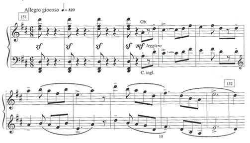
The use of these so-called open intervals lends a simple, elemental character to the music. Thus, whether used in the same way as in folk music or not, these intervals are able easily to invoke in the listener thoughts of folk music.
It is no surprise that the octave is the most numerous of the larger intervals, or that there are few intervals larger than an octave. These tendencies have been true of melodic style for generations. What is different from traditional style, however, is the greater number of large descending intervals compared to large ascending intervals.
Summary
In summary, the melodies of Romeo and Juliet, although based on diatonic scales, contain a high number of chromatic pitches. This high use of chromaticism is closely linked with a willingness on Prokofiev's part to follow, on occasion, any note with almost any other. On the other hand, most tones show strong tendencies toward particular resolutions, some traditional, some, especially in the case of chromatic pitches, new. Conjunct motion is preferred. A high incidence of fourths and fifths is observed, as well as a low incidence of tritones, two features not common to much other chromatic twentieth-century music.
The application of chi-square tests and Joseph Youngblood's information-theory techniques to the melodies of Romeo and Juliet points to enough obvious facts to demonstrate the validity of the methods. The assertion shown by the chi-square test that the Prokofiev melodies are significantly more chromatic than Schubert's, for instance, is just the result we would expect, as is the judgment from information theory that the entropy for Romeo and Juliet's major melodies is lower than that of all the melodies together. On the other hand, the tests reveal some less intuitive facts, showing the methods' usefulness: the tendency of 1 to precede 5, for instance, or the tendency of 10 to precede 11. While these kinds of melodic details form only one part of the complex system known as a style, they form a significant part, singled out by Meyer in his explanation of "embodied meaning." (See quotation by Meyer on the first page of this article.) In response to Meyer's implication in that quotation that style involves systems of probabilities for more than just the immediately forthcoming note, the present study seeks to extend Youngblood's method to pairs separated by one note, and with some success: the absence of inclination toward delay of note-to-note tendencies and particular findings such as the tendency of both 6 and 10 to return two notes later are surprising and thus significant.
What are we to make of these findings? As I mentioned earlier, any kind of note-counting technique should be taken only as a first step toward understanding. The work may be built upon in two ways. First, further studies could, by using this baseline, examine relationships between the style of these melodies and others. Just as the purpose of this study is to compare one style usually dubbed "tonal" with others by means of the baseline offered by Youngblood, the tendencies revealed here might be used as a frame of reference within which to examine melodies by other twentieth-century neotonal composers, or even other melodies by Prokofiev, thus perhaps revealing aspects of the development of his style. Second, an increased enjoyment of Romeo and Juliet should not be dismissed as an insignificant by-product of the study: the results of the statistical tests run here may be used as the basis for a more engaged hearing of the music. As Meyer points out, for a listener acquainted with a style, static probabilities become active expectations.
1Joseph E. Youngblood, "Style as Information," Journal of Music Theory 2 (April 1958): 24-35.
2Leonard B. Meyer, "Meaning in Music and Information Theory," The Journal of Aesthetics and Art Criticism 15 (June 1957): 412-424; reprinted as chapter 1 in Music the Arts and Ideas (Chicago: University of Chicago Press, 1967).
3Meyer, "Meaning in Music," 413.
4Meyer, "Meaning in Music," 414.
5Meyer, "Meaning in Music," 422.
6The source for these melodies and for the excerpt given as example 1 is Sergei Prokofiev, Romeo and Juliet, Piano Score (Melville, NY: Belwin Mills, n.d.). Locations in the score are identified using a measure number as counted from the appropriate rehearsal number. (100:5 refers to the fifth measure after rehearsal number 100.)